A brief introduction to EEG & ERP
Created: 2025-01-29
What is EEG?
Electroencephalography (EEG) records electrical activity produced by (populations of) neurons
Measured through electrodes placed on the scalp
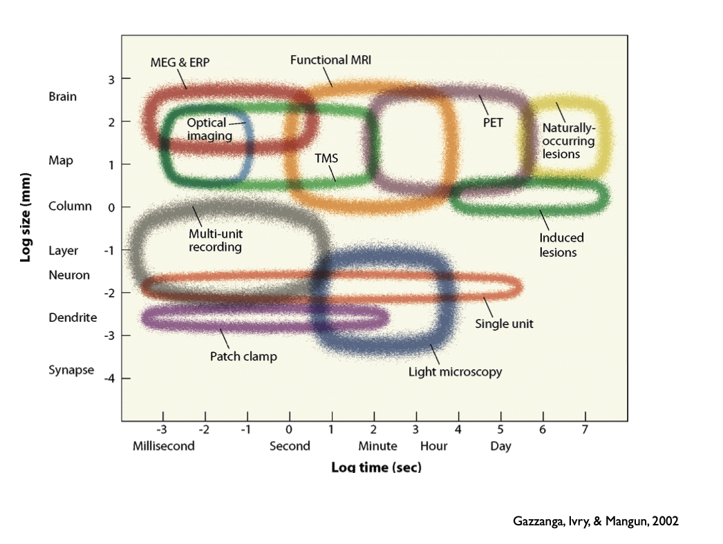
Captures real-time brain activity with millisecond precision
Non-invasive, relatively inexpensive method
Historical Development
Hans Berger records first human EEG (1929)
- First human neuroimaging technique
Pauline and Hallowell Davis credited with first observations of auditory evoked ERPs in 1936
Jasper 1937, first visual ERPs
Walter et al. (1964) first report of the CNV (contingent negative variation, a frontal negative potential representing anticipatory attention)
1960s-1970s, new computational techniques leads to ERP methodology (averaging)

Cellular Basis of EEG
Pyramidal neurons are the main source of EEG signals
Large cortical neurons oriented perpendicular to surface; dendrites extend toward cortical surface
Synchronized postsynaptic potentials create measurable fields, polarity depending on orientation of cortical surface
- Scalp-recorded potentials only possible for layered structures with consistent orientations, i.e. primarily cerebral cortex
Requires ~10,000 neurons firing together to generate detectable signal –> low spatial resolution
EEG Frequency Bands
Delta (0.5-4 Hz): Deep sleep
Theta (4-8 Hz): Drowsiness, meditation
Alpha (8-13 Hz): Relaxed wakefulness
Beta (13-30 Hz): Active thinking
Gamma (>30 Hz): Complex processing
EEG vs fMRI
| EEG | fMRI | |
|---|---|---|
| Temporal resolution | Good (in milliseconds) | Low (in seconds) |
| Spatial resolution | Poor (in centimeters) | High (in 1-2mm voxels) |
| Cost | Low relative to fMRI | Very high |
| Portability | Portable systems available | Requires fixed, dedicated installation |
| Comfort | Minimal discomfort | Loud, may be claustrophobic |
| Motion sensitivity | Moderate | High |
| Measured activity | Direct measurement of neuronal electrical activity | Indirect measurement via blood oxygen levels (BOLD signals) |
| Limitations | Low spatial resolution Only measures cortex |
Low temporal resolution |
Modern EEG Recording Systems
Ag/AgCl electrodes most common
Electrode-skin interface:
- Conductive gel reduces impedance
Signal acquisition parameters
- Sampling rate: typically 250-2000 Hz
- Analog-to-digital conversion: 16-24 bit
- Amplification: 1000-100,000x gain
- Online filtering: high-pass 0.1-1 Hz; low-pass ~100-200 Hz
- Notch: 50/60 Hz (power line)
BioSemi ActiveTwo vs. Brain Products actiCHamp
| Feature | BioSemi ActiveTwo | Brain Products actiCHamp |
|---|---|---|
| Active Electrodes | Yes (Active Pin-Type) | Yes (actiCAP active) |
| Reference Scheme | CMS/DRL feedback loop | Traditional reference |
| Max Channels | 256 | 160 |
| Sampling Rate | Up to 16384 Hz | Up to 100 kHz |
| Resolution | 24-bit | 24-bit |
| Input Range | ±262 mV | ±400 mV |
| Bandwidth | DC to 3.2 kHz | DC to 7.5 kHz |
| Interface | USB2/Optical fiber | USB |
| Battery Operation | Yes | No (USB powered) |
| Trigger Input | 16-bit parallel | 8-bit parallel/serial |
| Special Features | Zero reference design Replaceable electrode tips Active shielding |
Impedance measurement Built-in calibration Electrode position detection |
| Software | ActiView | BrainVision Recorder |
Sources of Noise in EEG Recordings (1/2)
Biological Artifacts
- Muscle activity (EMG)
- High frequency (>20 Hz)
- Preventive: participant relaxation
- Analysis: ICA, high-pass filtering
- Eye movements & blinks
- Large amplitude deflections
- Preventive: eye movement controls
- Analysis: ICA, regression-based correction
- Cardiac activity (ECG)
- Regular rhythmic activity
- Analysis: ICA, template matching
Environmental Noise
- Power line interference (50/60 Hz)
- Preventive: Proper grounding
- Analysis: Notch filter
- Electronic equipment
- Preventive: Shield recording area
- Keep electronics away from EEG system
Sources of Noise in EEG Recordings (2/2)
Technical Noise
- Electrode issues
- Poor contact: Check impedance
- Bridging: Do not overgel
- Cable movement: Secure cables
- Amplifier noise
- Regular calibration
- Proper maintenance
- Temperature stability
Handling Noise
- Prevention during recording:
- Proper shielding
- Subject instruction
- Equipment maintenance
- Regular impedance checks
- Analysis solutions:
- Filtering (appropriate frequency bands)
- Artifact rejection
- ICA decomposition
- Robust averaging techniques
- Reference choice optimization
Event-Related Potentials
Time-varying neural responses to specific events
Events could be external stimuli, or
Participant internal activity (visual, cognitive processing)
Relies on
- Consistent marking of the events
- Averaging, to remove noise independent of (cannot be removed by) pre-processing
ERPs are latent structures
Examples:
N100: Early sensory processing
P200: Feature detection
N200: Stimulus discrimination
P300: Target detection, decision-making
N400: Semantic processing
Event-Related Potentials: Example


Anatomy of an ERP Component
Polarity: Positive (P) / Negative (N)
- Depends on: neurotransmitter type (excitatory/inhibitory), synapse location, orientation of cortical surface, superposition of other sources
- Polarity alone has no inherent meaning
- Same cognitive process can produce different polarities at different sites - positive ≠ excitation, negative ≠ inhibition
Amplitude: Size of deflection (μV)
- Depends on: number of neurons activated, geometry of neurons, synchronicity of post-synaptic potentials, depth of source, orientation of cortical surface, superposition of other sources
- Voltage peaks are not the same as components!
Latency: Time from stimulus onset (ms)
Duration: Time course of the component
Topography: Scalp distribution
Interpreting ERP components (1/2)
Common Mistakes
Single component ≠ single process
Differences in peak amplitude ≠ change in component size
Larger amplitude of a component ≠ “more processing”
Peak latency ≠ process duration
Over-interpreting scalp distribution
Confusing correlation with causation
Average ERP may not reflect what happens on individual trials
Ignoring component overlap
Interpreting ERP components (2/2)
Component Overlap
An effect in one time period doesn’t necessarily mean a modulation of the component at that time period.
Difference waves can sometimes reveal the underlying component time course
Later components affected by earlier ones
Solutions:
Use difference waves
Principal Component Analysis (PCA)
Independent Component Analysis (ICA)
Careful experimental design to remove confounds
Component Overlap


Best Practices in ERP Research
Use appropriate control conditions
Maintain consistent trial numbers
Consider individual differences
Document and report all pre-processing steps
Use standardized electrode positions
Document analysis parameters
Consider alternative explanations
Considerations for Experimental Design
Sufficient trial numbers (>30-40 per condition)
Balanced conditions
Appropriate inter-stimulus intervals
Control for:
Physical stimulus properties
Motor responses
Attention and arousal
Order effects
Basic ERP data pipeline
- Reference
- Filter
- Artifact rejection
- Epoch
- Baseline correction
- Averaging across trials (single subject)
- Grand averaging across subjects
Questions?
Thank you for your attention!